Symbolic Computations
Symbolic Computations
Neil J. Gunther
Contents
1 Mathematical Animation
2 Earth's Curvature
3 The Batman Equation
3.1 Original Equation in MMA
3.2 Modified Equation in MMA
4 Feynman's Quantum Mechanics
4.1 Cornu Spiral
4.2 Youngian Interference
4.3 References
5 Visual Riemann Hypothesis
5.1 Cube Roots of Unity
5.2 5th Roots of Unity
5.3 11th Roots of Unity
5.4 17th Roots of Unity
5.5 61st Roots of Unity
5.6 Generalized Equation
5.7 Tabulated Comparison
6 Hydrogen Spectrum
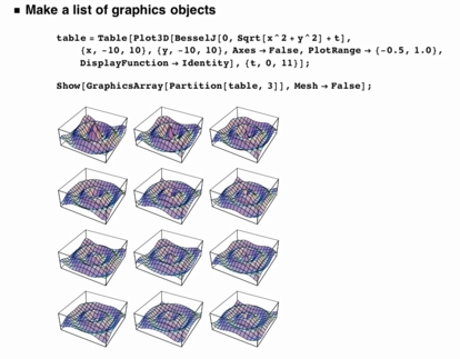
1 Mathematical Animation
Nothing deep but, being my first attempt at animation, is was very exciting to see it come to life
in Mathematica.
Made with Mathematica 4.1 on Wed Oct 24 01:13:59 2001
2 Earth's Curvature
A scaled simulation of the apparent increase in the curvature of the
Earth's horizon as the altitude of a virtual observer increases from 30
feet to 30 miles. This is similar to the view an astronaut would have
during a rocket launch.
 |
| A view the Earth's horizon from an altitude of 30 miles. |

|
Made with Mathematica 4.1 on Wed Jun 19 21:39:47 2002
3 The Batman Equation
Having recently posted my
winking pink elephant in R,
I had my attention directed to this posting about the
Batman equation.
Naturally, I couldn't resist spending "a few minutes" trying it out in Mathematica.
The intent of the Batman equation (I assume)
is to represent Tim Burton's 1989 movie logo
in mathematical form. As usual, there's more to it than meets the eye and it cost me more than a few minutes.
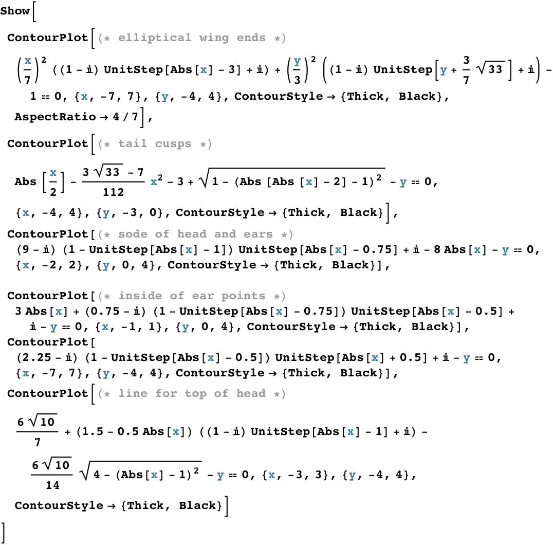
3.1 Original Equation in MMA
The simplest thing seemed to be to try rendering the equation verbatim using the ContourPlot function in MMA.
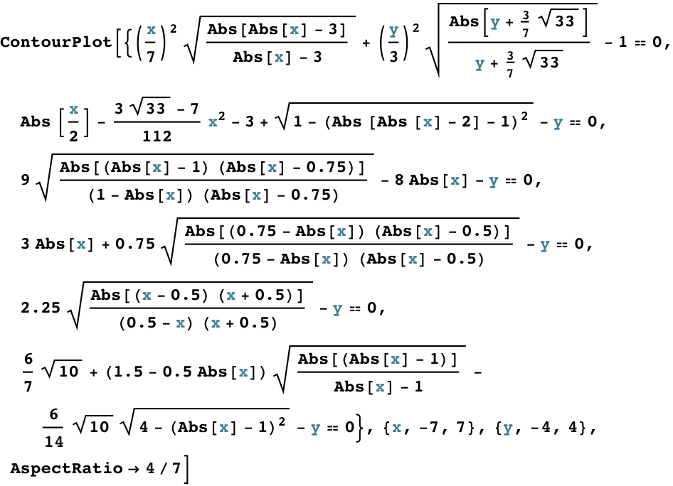
Because the ContourPlot function plots regions by default, I entered each factor as a separate equation (using == 0).
But it turns out not to make any difference in this particular construction.
The more important point is that the resulting plot (Fig. 1) has "noise" due to lack of
numerical cancellations and there are some missing line segments (viz., the pointy ears). Also, each factor
in the overall equation can be quite sensitive to the domain of values in the computation.
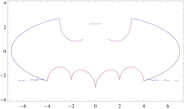 Figure 1: Plot produced by the MMA code.
3.2 Modified Equation in MMA
While investigating how to get rid of the noise problems (assuming it wasn't an MMA bug), I realized that the role of
the radicals in the original equation is to switch the numerical values from purely real numbers to complex numbers
(numbers of the form a + ib) by adding an imaginary ib component to the number. The idea is that points in the xy-plane are all real-valued.
An imaginary component of a complex number can be thought of as a value in the z-direction, pointing out of the xy-plane.
Therefore, a purely imaginary number will sit above the plane and won't be plotted.
That's how segments of the various curves are switched off or truncated in the Batman plot.
Cute trick, but what happens if the complex number a + ib is such that a is big while b is relatively tiny?
ContourPlot has to decide whether or not to plot that point. You see how the noise troubles can creep into Figure 1.
Similarly, the computation of square roots can present numerical problems. To avoid all this, I discovered a way of
replacing the radicals of the rational functions with the following identity:
|
A |
√
|
| (A − |x|) (|x| − B) |
(A − |x|) (|x| − B)
|
|
= [ A − i (1 − U(|x| − A) ] U(|x| − B) + i |
| (1) |
where A and B are constants, U is the UnitStep function
in MMA and i = √(−1).
The modified MMA code using eqn.(1) becomes:
and the resulting plot looks like this
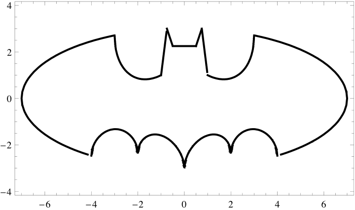 Figure 2: Plot produced by my modified MMA code.
I think the little discovery of eqn.(1) made the time spent well worth it. :)
Made with Mathematica 7 on Sat, Jul 30, 2011
4 Feynman's Quantum Mechanics
Feynman's formulation of quantum mechanics (QM) [1]
and quantum electrodynamics (QED) [2] is based on the complicated
mathematics of functional integrals over space-time paths.
A simpler way of appreciating the underlying mathematics
is to think of a quantum particle, like
an electron or photon, as belonging to an arrow which rotates at the
frequency ν corresponding to its energy (E = hν)
as it moves from emitter, e.g., a laser to a detector, e.g., CCD camera [3, 4]. The difference between a classical particle
(like a ball bearing) and a quantum particle is that the former traverses only one possible path (the classical
path) in space-time, whereas the latter traverses all possible paths. The summation over all these paths
corresponds to the functional integral.
When they reach the CCD image-plane or detector, the arrows belonging to
all these paths stop rotating. The procedure then is to determine the
length of the resultant arrow by adding all the individual
path-arrows vectorially (i.e., head-to-tail). Squaring the length of the
resultant arrow gives the probability of finding the quantum particle at
that location in the image-plane or detector. From a classical wave-theory point of view,
it corresponds to the intensity of the light at that point.
A nice visual example of this procedure is provided by the
Cornu spiral,
which accounts for why a point of light in a photograph is slightly fuzzy rather than sharp.
4.1 Cornu Spiral
Figure 3 shows how to compute the Cornu spiral using Feynman's arrows [3 p. 57].
The left side of Figure 3 shows the point source and a point in the detector or vertical image plane.
Midway is a set of vertical dots that represent a
diffraction grating.
The photon takes all paths between its
source and each vertical dot, and similarly from the dots to the detector point. Note that it's the same
physical photon that takes all these paths simultaneously. Weird, but that what makes it a quantum particle
and not a classical particle.
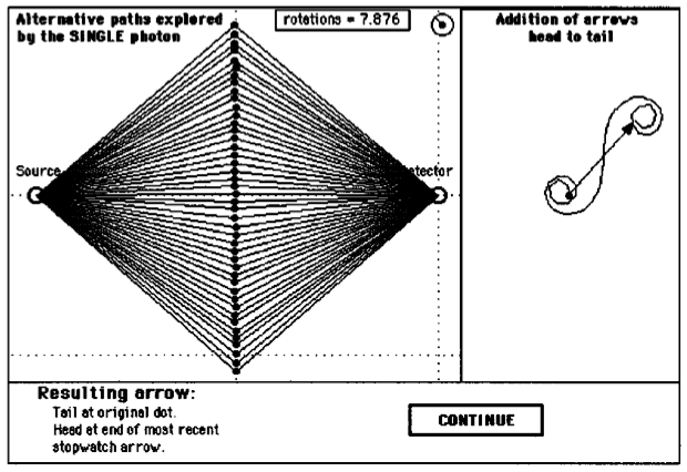 Figure 3: Computing the Cornu spiral using Feynman's arrows. From [5]
The rotating arrows from all these paths arrive at the detector point and stop rotating.
They are then added vectorially as shown on the right panel in Figure 3.
The large resultant arrow is shown pointing roughly north-east.
The same explanation, without any reference to QM, appears in [6, p. 30-9]
If the diffraction grating is replaced by a converging lens, then all the
arrows would reach the image plane at the same time, and the "curly ends"
of the Cornu spiral would staighten out to produce a longer resultant arrow
[3, p. 58]. Physically, that corresponds to a brighter sharper
image; which is why we use lenses.
4.2 Youngian Interference
In 1803,
Thomas Young
(he also of Rosetta stone fame) presented the results of a simple
double-source interference
experiment which helped to convince the scientific world that light was a wave phenomenon, thus supporting Huygen's
model rather than Newton's corpusular model of light. But Newton's particle was actually closer to
the modern QM model of the photon.
As Feynman explains in lecture 4b, Newton got totally hosed up
trying to explain partial reflections because he was thinking in terms of a classical particle rather than
a quantum particle.
Thus, Newton had to resort to anthropomorphic terms like the corpuscle throws a "fit" to
account for certain effects.
Figure 4 shows the result of my
MMA
computation of
2-slit interference
using Feynman's arrows. The asymmetry of the arrows about the origin, relative to the symmetry of the
squared amplitude, is a notable curiosity.
Ironically, Youngian interference is not discussed explicitly in [3], but
Feynman does employ it explicitly (with electrons) to motivate
the more mathematical treatment in [1].
I suspect the reason for this is that interference is expected for light,
because light is always introduced in the context of a wave phenomenon (Huygens, Maxwell) whereas,
electron interference seems counterintuitive, because electricity is associated with the Coulomb charge unit
or molar electrolysis.
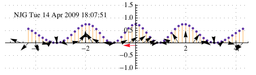 Figure 4: Double slit interference. When the path-arrows are added and squared, they produce the
sinusoidal pattern of dots which corresponds to the probability of finding the photon at that location
in the image plane. Unlike Figure 3, I've oriented the image plane horizontally.
Figure 4: Double slit interference. When the path-arrows are added and squared, they produce the
sinusoidal pattern of dots which corresponds to the probability of finding the photon at that location
in the image plane. Unlike Figure 3, I've oriented the image plane horizontally.
A similar explanation, without any reference to QM, appears in [6, p. 29-5 and Chapter 30].
4.3 References
-
R. P. Feynman and A. R. Hibbs, Quantum Mechanics and Path Integrals,
McGraw-Hill, New York, 1965.
-
R. P. Feynman, Quantum Electrodynamics,
W. A. Benjamin, Mass., 3rd printing, 1973.
-
R. P. Feynman, QED, The Strange Theory of Light and Matter,
Princeton University Press, Princeton, 1985.
-
Streaming video of Feynman lecturing on QED at the University of Auckland, New Zealand in 1979:
- Photons - Corpuscles of Light
-
Fits of Reflection and Transmission
- Electrons and Their Interactions
- New Queries
This material is essentially identical to that published in the QED book [3].
-
E. F. Taylor, S. Vokos, J. M. O'Meara and N. S. Thornberd,
"Teaching Feynman's sum-over-paths quantum theory,"
COMPUTERS IN PHYSICS, VOL. 12, NO. 2, MAR/APR 1998.
-
R. P. Feynman, R. Leighton, and M. Sands, The Feynman Lectures on Physics, Vol. 1,
Addison-Wesley, 6th printing, 1977. Also available as video at
Microsoft but
requires their Silverlight browser plug-in.
Made with Mathematica 7 on Tue, Apr 14, 2009
5 Visual Riemann Hypothesis
If it could be proven,
the Riemann hypothesis (RH)
would explain the
distribution of the prime numbers.
One statement of RH says that all the nontrivial zeros of the Riemann zeta function ζ(s) in the complex plane,
lie on the critical line with Re(s) = 1/2.
According to Brian Conrey in this
lecture,
an associated graphical interpretation of RH can be constructed using arrows which are added vectorially.
The
285 MB Windows Media Player file
is available for download.
The relevant section starts at 47:30 minutes.
You may need to turn up the volume because the sound quality is rather poor.
Unfortunately, Conrey becomes confused when he describes the role of perfect squares in reversing the
direction of some arrows. I think this happens because he tries to oversimplify it. It's not that the relevant
numbers are perfect squares but rather,
quadratic residues or remainders of p.
Conrey, being a number theorist, clearly understands this because he has the
correct list of quadratic residues along the bottom of his slides; it's just that he
fumbles the explanation.
Since the graphical construction is very simple, especially when compared with the deeper mathematical
significance of RH, it is worth understanding correctly. What follows, is my version of what
he is describing.
5.1 Cube Roots of Unity
Conrey starts with p = 5 but I think it's easier to see the principle behind the graphical construction
using the first odd prime p = 3.
 Consider its 3
roots of unity as 3 vectors
in the complex plane.
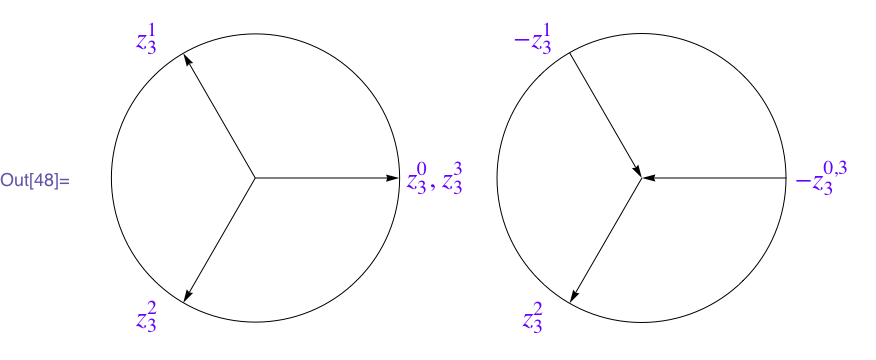
Next, we make a list of indices that correspond to the quadratic residues mod 3.
Consider its 3
roots of unity as 3 vectors
in the complex plane.
Next, we make a list of indices that correspond to the quadratic residues mod 3.
- 12 = 1 (mod 3)
- 22 = 1 (mod 3)
So, 1 is the only unique residue mod 3, which
means we take the vector corresponding to z13 and reverse it's direction.
By convention, we also do the same thing with the z03 vector. Now, we add the vectors head-to-tail as
shown in the following diagram.
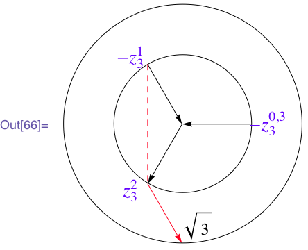
We find that the end-point (the red arrowhead) lands on a circle of radius r = √3 = 1.73205,
which is the square root of our starting prime number.
5.2 5th Roots of Unity
Start with p = 5 (Conrey's first example in the movie) and determine the quadratic residues mod 5:
- 12 = 1 (mod 5)
- 22 = 4 (mod 5)
- 32 = 4 (mod 5)
- 42 = 1 (mod 5)
The unique residues are therefore 1 and 4, and
we see they correspond to the reversed arrows in Conrey's diagram.
Adding the arrows vectorially, we end on a circle of radius √5.
5.3 11th Roots of Unity
Choosing p = 11, we can use this
Java-based calculator
to do determine the unique residues:
Quadratic residues modulo 11:
1, 3, 4, 5, 9
There are 5 quadratic residues modulo 11.
Switching the direction of these arrows and adding them vectorially,
we end on a circle of radius √11 as shown in Figure 5.
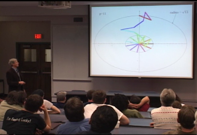 Figure 5: Brian Conrey showing how the addition of vectors for the case of p = 11 ends on a circle with
radius √11. That the circles look like ellipses in the picture
is presumably due to incompatible aspect ratio settings
between his PC screen and the digital projector display.
Figure 5: Brian Conrey showing how the addition of vectors for the case of p = 11 ends on a circle with
radius √11. That the circles look like ellipses in the picture
is presumably due to incompatible aspect ratio settings
between his PC screen and the digital projector display.
5.4 17th Roots of Unity
Starting with p = 17, we have:
Quadratic residues modulo 17:
1, 2, 4, 8, 9, 13, 15, 16
There are 8 quadratic residues modulo 17.
such that we end on a circle of radius √17
5.5 61st Roots of Unity
If we start with p = 61 (Conrey's final example), reverse the following vectors:
Quadratic residues modulo 61:
1, 3, 4, 5, 9, 12, 13, 14, 15, 16, 19, 20, 22, 25, 27, 34, 36, 39, 41,
42, 45, 46, 47, 48, 49, 52, 56, 57, 58, 60
There are 30 quadratic residues modulo 61.
and add them vectorially, we end on a circle of radius √61.
This works for any prime number!
The √p radical can also be written as an exponent p1/2 and, according to Conrey,
that is associated with the critical line at Re(s) = 1/2 in RH.
5.6 Generalized Equation
I discovered that I could express this vector addition in equational form:
|
|
p−1
∑
k=1
|
(k | p) exp |
|
i |
2 π k
p
|
|
|
= p1/2 |
| (2) |
where (k | p) is the Legendre symbol.
The Legendre symbol automatically handles reversing the appropriate vectors—which is very cool.
Equation (2) can be written as an
MMA function:
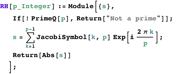
The Legendre symbol is just a special case of the
Jacobi symbol in MMA.
The symbolic output for p = 29 is:
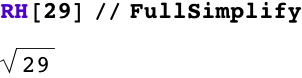
in agreement with Conrey's diagrammatic scheme.
5.7 Tabulated Comparison
Since the symbolic simplification can become compute-bound for larger primes, it is faster just to
compare numerical output. We can take a selection of p values from the
first 100 prime numbers,
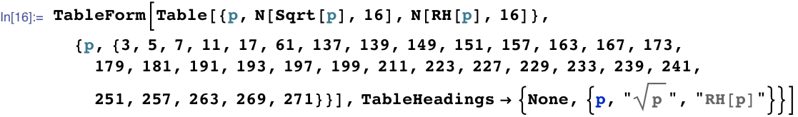
to show that the results agree numerically.
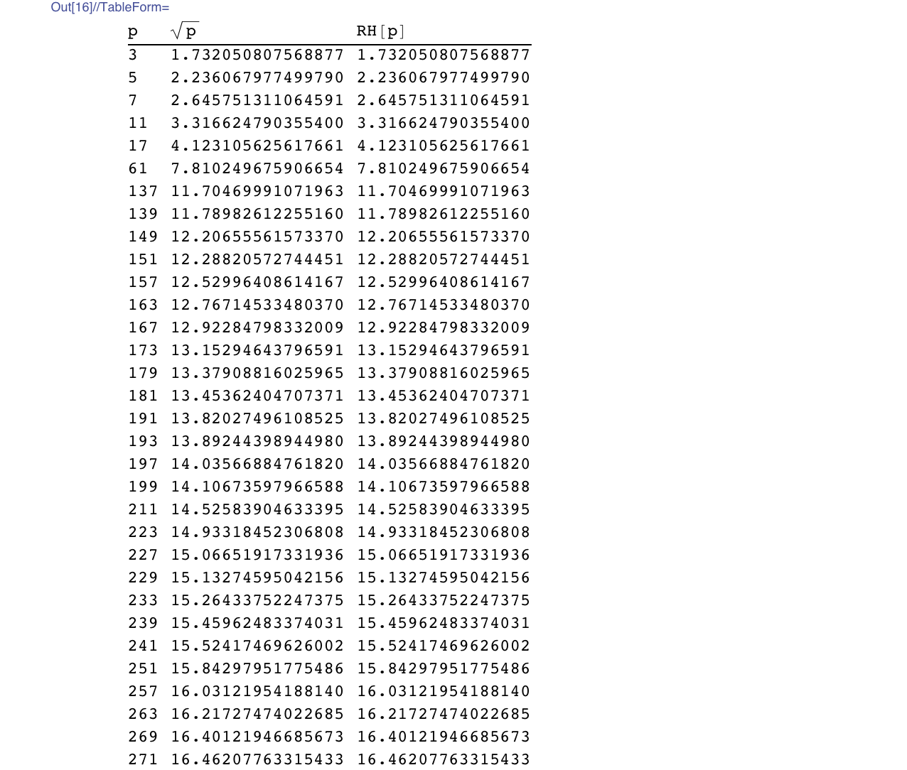
By now, you might be thinking this is all a bit obvious, but it's not. We are not doing simple vector addition
of the prime-th roots of unity. There is no way eqn. (2) can work without
the reversing the correct vectors. So, the secret really lies in the Legendre symbol.
In fact, eqn. (2) is essentially the discrete Fourier transform of the Legendre symbol.
Made with Mathematica 7 on Wed, Aug 4, 2010
6 Hydrogen Spectrum
This project is still under construction.
Semiclassical orbital rosette.
Comparison on spectral models.
Made with Mathematica 7 on Wed, July 6, 2011
File translated from
TEX
by
TTH,
version 3.81.
On 3 Nov 2017, 10:30.